Thursday, December 31, 2009

DataStage PX Training.


Administrator Module
Manager Module
Designer Module
Director Module
Parallelism Concepts

Adminstrator Module
Upon module completion, you will be able to:
Create and remove projects
Set project-level properties
Set environment variable default values and add new variables and values, if necessary


Logging into a DataStage server using the Administrator requires the host name of the server—the fully qualified name if necessary—or the server’s IP address, and an operating system username and password. For UNIX servers, users logging in as root or as a root-equivalent account, or as dsadm will have full administrative rights. For Windows servers, users logging in who are members of the Local Administrators (standalone server) or Domain Administrators (domain controller or servers in an Active Directory Forest) groups will have full administrative rights.

This page lists the DataStage projects, and shows the pathname of the selected project in the Project pathname field. The Projects page has the following buttons:

• Add… adds new DataStage projects. This button is enabled only if you have administrator status.
• Delete deletes projects. This button is enabled only if you have administrator status.
• Properties views or sets the properties of the selected project.
• NLS… lets you change project maps and locales (if the NLS option was installed during the server installation).
• Command issues DataStage Engine commands directly from the selected project.


Provided that you have the proper permissions, you can add as many projects to the DataStage server as necessary. In normal projects any DataStage developer can create, delete, or modify any object within the project once it has been created. During the creation process, however, you can specify that a new project is protected. This is a special category of project and, normally, nothing can be added, deleted or changed in the project. Users can view objects in the project, and perform tasks that affect the way a job runs rather than the jobs design; specifically they can:
• Run jobs
• Set job properties
• Set job parameter default values.

A newly created protected project is populated by importing developed jobs and components; only a Production Manager user can perform the import, no other types of user can import into a special project.

Tip: The default directory path in which to create projects is located under the root directory of the DataStage server installation. For example, if the server was installed to /appl/Ascential/DataStage the projects would be installed to /appl/Ascential/DataStage/Projects/{project name}. If a separate UNIX file system or Windows partition is available and has enough free space (refer to the DataStage Install and Upgrade Guide for project sizing values), change the path to reflect the proper location on the server before creating the new project. As you will see later on in the course, too many projects in the same file system or partition can lead to problems with free space—which can ultimately lead to the engine malfunctioning.


Provided you have the proper permissions, you can delete any project from the DataStage server. Before you delete any project, you should be sure that you have a proper backup of the project. This can be done from the DataStage Manager and is discussed in the Manager Module.


From the General tab, you can set some basic properties for the project:
Enable job administration in Director—enabling this feature will allow users the ability to Cleanup Resources and Clear Status File from within the Job menu of DataStage Director. The features let DataStage users release the resources of a job that has aborted or hung, and so return the job to a state in which it can be rerun when the cause of the problem has been fixed. Users should proceed with caution when cleaning up resources, since the utility will allow users to view and end job processes and view and release the associated locks of those processes. Also, remember that users can only end processes or locks that they own—some processes and locks will require administrative authority to clear them.
Enable Runtime Column Propagation for Parallel Jobs—if you enable this feature, stages in parallel jobs can handle undefined columns that they encounter when the job is run, and propagate these columns through to the rest of the stages in the job. This check box enables the feature; to actually use it you must explicitly select or deselect the option on each stage. If it is enabled, all stages in parallel jobs will have RCP enabled as a default setting. This setting has no effect on jobs created on the server canvas.
Auto-purge of job log—this setting will automatically purge job log entries for jobs based on the auto-purge action setting. For example, if you specify to auto purge up to the previous 3 job runs, entries for the previous 3 job runs are kept as new job runs are completed. Keep in mind that the auto purge setting applies to newly created jobs, not existing jobs. If you want to enable the auto-purge setting for a previously created job, this can be accomplished from the DataStage Director.


You can set project-wide defaults for general environment variables or ones specific to parallel jobs from this page. You can also specify new variables. All of these are then available to be used in jobs. In each of the categories except User Defined, only the default value can be modified. In the User Defined category, users can create new environment variables and assign default values.


You can trace activity on the server to help diagnose project problems. The default is for server tracing to be disabled. When you enable it, information about server activity is recorded for any clients that subsequently attach to the project. This information is written to trace files, and users with in-depth knowledge of the system software can use it to help identify the cause of a client problem. If tracing is enabled, users receive a warning message whenever they invoke a DataStage client.

You can also view or delete current trace files from within this window by selecting the trace file and clicking on view or delete.


This tab applies to Windows NT/2000 servers only. DataStage uses the Windows NT Schedule service to schedule jobs. This means that by default the job runs under the user name of the Schedule service, which defaults to NT system authority. You may find that the NT system authority does not have enough rights to run the job. To overcome this, you can specify a user account and password to run DataStage jobs in a project under that user’s authority. Click Test to test that the user name and password can be used successfully. This involves scheduling and running a command on the server, so the test may take some time to complete.


Hashed file stage caching: When a Hashed File stage writes records to a hashed file, there is an option for the write to be cached rather than written to the hashed file immediately. Similarly, when a Hashed File stage is reading a hashed file there is an option to pre-load the file to memory, which makes subsequent access much faster and is typically used when the file is providing a reference link to a Transformer stage.

Row buffering: The use of row buffering can greatly enhance performance in server jobs. Select the Enable row buffer check box to enable this feature for the whole project. There are two types of mutually exclusive row buffering:
• In process. You can improve the performance of most DataStage jobs by turning in-process row buffering on and recompiling the
job. This allows connected active stages to pass data via buffers rather than row by row.
• Inter process. Use this if you are running server jobs on a multi-CPU server (SMP). This enables the job to run using a separate process for each active stage, which will run simultaneously on a separate processor.

When you have enabled row buffering, you can specify the following:
• Buffer size. Specifies the size of the buffer used by in-process or inter-process row buffering. Defaults to 128 Kb.
• Timeout. Only applies when inter-process row buffering is used. Specifies the time one process will wait to communicate with another via the buffer before timing out. Defaults to 10 seconds.

Job Parameters

* Defined in job Properties window
* Makes the job more flexible
* Parameters can be:
- Used in directory and file names
- Used to specify property values
- Used in constraints and derivations
* Parameter values are determined at run time
* When used for directory and files names and property
Vlues, they are surrounded with pound signs(#)
- E.g., #NumRows#
* Job parameters can reference DataStage environment variables
- Prefaced by $, e.g., $APT_CONFIG_FILE
-----------------------------------------------------------------
Running Jobs from Command Line

* dsjob -run -param numrows=10 dx0863 GenDataJob
- Runs a jo b
- Use -run to run the job
- Use -param to specify parameters
- In this example, dx0863 is the name of the project
- In this example, GenDataJob is the name of the job
* dsjob -logsum dx0863 GenDataJob
- Displays a job's messages in the log
------------------------------------------------------------------
Runtime Column Propagation ( RCP )

* When RCP is trurned on:
- Columns of data can flow through a stage without being explicitly defined in the stage
- Target columns in a stage need not have any columns explicitly mapped to them
* No column mapping enforcement at design time.
- Input columns are mapped to unmapped columns by name.
* How implicit columns get into a job
- Read a file using a schema in a sequential file stage
- Read a database table using "Select * "
- Explicitly define as a n output column in a stage earlier in the flow

Benefits of RCP
- Job flexibility
* Job can process input with different layouts
- Ability to create reusable components in shared containers
* Component logic an apply to a single name column
* All other columns flow through untouched.

Enabling Runtime Column Propagation ( RCP )

# Project level
- DataStage Administrator Parallel tab.
# Job level
- Job properties General tab.
# Stage level
- Link Output Column tab.
# Setting at a lower level override settings at a higher level.
- E.g., disable at the project level, but enable for a given job.
- E.g., enable at the job level, but disable a given stage.

Datastage PX certification

1)Which two statements are correct about XML stages and their usage? (Choose two.)
A. XML Transformer stage converts XML data to tabular format.
B. XML Input stage converts XML data to tabular format.
C. XML Output stage uses XSLT stylesheet for XML to tabular transformations.
D. XML Output stage converts tabular data to XML hierarchical structure.

2)Which two statements are true about usage of the APT_DISABLE_COMBINATION environment
variable? (Choose two.)
A. Globally disables operator combining.
B. Must use the job design canvas to check which stages are no longer being combined.
C. Disabling generates more processes requiring more system resources and memory.
D. Locks the job so that no one can modify it.

3)When importing a COBOL file definition, which two are required? (Choose two.)
A. The file does not contain any OCCURS DEPENDING ON clauses.
B. The column definitions are in a COBOL copybook file and not, for example, in a COBOL source
file.
C. The file you are importing contains level 01 items.
D. The file you are importing is accessible from your client workstation.

4)A client requires that any job that aborts in a Job Sequence halt processing. Which three activities
would provide this capability? (Choose three.)
A. Exception Handler
B. Nested Condition Activity
C. Job trigger
D. Sendmail Activity
E. Sequencer Activity

5)A DataStage EE job is sourcing a flat file which contains a VARCHAR field. This field needs to be
mapped to a target field that is a date. Which task will accomplish this?
A. Use a Modify stage to perform the type conversion.
B. Perform a datatype conversion using DateToString function inside the Transformer stage.
C. Use a Copy stage to perform the type conversion.
D. DataStage automatically performs this type conversion by default.

6)You are reading data from a Sequential File stage. The column definitions are specified by a
schema. You are considering whether to follow the Sequential File stage by either a Transformer
or a Modify stage. Which two criteria require the use one of these stages instead of the other?
(Choose two.)
A. You want to dynamically specify the name of an output column based on a job parameter,
therefore you select a Modify stage.
B. You want to add additional columns, therefore you select a Transformer stage.
C. You want to concatenate values from multiple input rows and write this to an output link,
therefore you select a Transformer stage.
D. You want to replace NULL values by a specified constant value, therefore you select a Modify
stage.

7)Which three actions are performed using stage variables in a parallel Transformer stage? (Choose
three.)
A. A function can be executed once per record.
B. Identify the last row of an input group.
C. Identify the first row of an input group.
D. A function can be executed once per run.
E. Lookup up a value from a reference dataset.

8)Which three UNIX kernel parameters have minimum requirements for DataStage installations?
(Choose three.)
A. MAXPERM - disk cache threshold
B. MAXUPROC - maximum number of processes per user
C. NOFILES - number of open files
D. SHMMAX - maximum shared memory segment size
E. NOPROC - no process limit

9)Which partitioning method would yield the most even distribution of data without duplication?
A. Random
B. Hash
C. Round Robin
D. Entire

10)Which environment variable controls whether performance statistics can be displayed in
Designer?
A. APT_NO_JOBMON
B. APT_PERFORMANCE_DATA
C. APT_PM_SHOW_PIDS
D. APT_RECORD_COUNTS
==================================================================================
Reading and writing null values in Datastage EE

There are a few considerations that need to be taken into account when handling nulls in Datastage:
All DSEE data types are nullable
Null fields do not have a value. Enterprise Edition NULL is respresented by a special value outside the range of any legitimate Datastage values
Nulls can be written to nullable columns only (this setting is specified in the column properties)
The Datastage job will abort when a NULL is to be written to a column which does not allow nulls
Nulls can be converted to or from a value. For instance, in a Sequential File stage the nulls need to be handled explicitly. A value which will be written instead of a null needs to be specified.
In a sequential source stage it is possible to specify values that will be converted to NULLs
A stage can ignore Null fields, can trigger an error or other defined action
----------------------------------------------------------------------------------
How to manage Datastage DataSets?

The Datastage DataSets can be managed in a few ways:
The Datastage Designer GUI (also available Manager and Director) provides a mechanism to view and manage data sets. It can be invoked in Tools -> Data set management
orchadmin command-line utility - a tool available on Unix which is able to list records and remove datasets (all component files, not just the header file)
dsrecords is command-line utility which lists number of records in a dataset
------------------------------------------------------------------------------------
What gets deployed when installing an Information Server Domain?

The following components are installed when deploying the IBM Infosphere Server Domain:
Metadata Server - which is installed on an WebSphere Application Server instance
Datastage server (or multiple servers) - may run on the parallel (EE) or server engine
Repository Database - DB2 UDB by default (available with the installation), however other RDBMS can be used
Information Server clients: Administration console, Reporting console, DS Administrator, DS Designer, DS Director
Information Analyzer
Business Glossary
Optionally: Rational Data Architect, Federation Server
------------------------------------------------------------------------------------
What is included in the configuration layers?


Configuration layers indicate what is installed on the IBM Infosphere installation server (layers are installed on the machine local to the installation).

The configuration layers include:
Datastage and Information Server clients
Engine - Datastage and other Infosphere applications
Domain - metadata server and installed product domain components
Repository database
Documentation
------------------------------------------------------------------------------------
What is the IBM Information Server startup sequence?


The Information Server startup sequence need to be preserved to avoid errors.

The startup steps are as follows:
Metadata Server startup - from the Microsoft Windows start menu (start the server option) or type startup serverx in the profile bin directory where serverx is the default name of the application server hosting the MetaData server
Start the ASB agent - by default it is set to start during the system startup. To start it manually, go to the Information Server folder in the Start menu and click Start the agent. It is only required when the Infosphere components (Datastage and Metadata server) work on different servers.
Execute Administration and Reporting consoles by clicking the Information Server Web Console icon.
Double click the DataStage and QualityStage client icon to begin the ETL development
----------------------------------------------------------------------------------
What privileges are required to run a parallel job?

To run a parallel job in Datastage, a user must have the following minimum permissions:
Read access to APT_ORCHHOME
Execute permissions on local programs and scripts
Read and Write access to the disk resources
----------------------------------------------------------------------------------
What is the default ip address and port for Information Server Web Console?

The Infosphere Information Server environment administration is done in the IBM Information Server Web Console, accessed via a web browser.
The default address is http://localhost:9080, where localhost should be replaced by a hostname or IP address of the machine that hosts the MetaData server and the default port 9080 can be adjusted if necessary.

The default web console webpage asks for user and password to log on. Those are login credentials specified during the installation and the administrator can manage the IDs in the console
-----------------------------------------------------------------------------------
What are datastage user roles?
Infosphere Datastage user roles are set up in the project properties in Datastage Administrator. To prevent unauthorized access, all Datastage users must have a user role assigned in the administrative console.

Each Datastage user can have one of the following roles assigned:
Datastage Developer - with full access to all functions of a Datastage projects
Datastage Operator - this users are allowed to run and manage released Datastage jobs
Datastage Super Operator - can browse repository (read-only) and open Designer client
Datastage Production Manager - creates and manages protected projects
-----------------------------------------------------------------------------------
What is the server-side tracing?
Infosphere Datastage server-side tracing is enabled and disabled in project properties in the tracing tab of the Datastage Administrator.
By default, server side tracing is disabled, because normally tracing is a system resources consuming option and causes a lot of server overhead.
When the server-side tracing is enabled, the information about all datastage server activity is recorded and written to trace files.
It is strongly recommended to use tracing only by experienced Datastage users or with the help of Datastage customer support.
-----------------------------------------------------------------------------------
Datastage imports and exports

All types of Infosphere Datastage objects (stored in a repository) can be easily exported into a file or imported into Datastage from a previously created export.

Main purpose of creating imports and exports are:
Projects and jobs backups
Maintaining and versioning
Moving objects between projects or datastage installations
Sharing projects and jobs between developers.
Imports and exports are executed from within the Datastage Client (in previous versions it was Datastage Manager).
To begin the export process, go to the Datastage and QualityStage Client menu and click Export -> Datastage components. Then select the types of objects to export and specify the details of an export file - path, name and extension (dsx or xml).
Keep in mind that the path to the export file is on the client machine, not the server.

Datastage EE configuration file

The Datastage EE configuration file is a master control file (a textfile which sits on the server side) for Enterprise Edition jobs which describes the parallel system resources and architecture. The configuration file provides hardware configuration for supporting such architectures as SMP (Single machine with multiple CPU , shared memory and disk), Grid , Cluster or MPP (multiple CPU, mulitple nodes and dedicated memory per node).

The configuration file defines all processing and storage resources and can be edited with any text editor or within Datastage Manager.
The main outcome from having the configuration file is to separate software and hardware configuration from job design. It allows changing hardware and software resources without changing a job design. Datastage EE jobs can point to different configuration files by using job parameters, which means that a job can utilize different hardware architectures without being recompiled.

The Datastage EE configuration file is specified at runtime by a $APT_CONFIG_FILE variable.

Configuration file structure
Datastage EE configuration file defines number of nodes, assigns resources to each node and provides advanced resource optimizations and configuration.

The configuration file structure and key instructions:
node - a node is a logical processing unit. Each node in a configuration file is distinguished by a virtual name and defines a number and speed of CPUs, memory availability, page and swap space, network connectivity details, etc.
fastname defines node's hostname or IP address
pool - defines resource allocation. Pools can overlap accross nodes or can be independent.
resource (resources) names of disk directories accessible to each node.
The resource keyword is followed by the type of resource that a given resource is restricted to, for instance resource disk, resource scratchdisk, resource sort, resource bigdata

Sample configuration files

Configuration file for a simple SMP
A basic configuration file for a single machine, two node server (2-CPU) is shown below. The file defines 2 nodes (dev1 and dev2) on a single etltools-dev server (IP address might be provided as well instead of a hostname) with 3 disk resources (d1 , d2 for the data and temp as scratch space).

The configuration file is shown below:

{
node "dev1"
{
fastname "etltools-dev"
pool ""
resource disk "/data/etltools-tutorial/d1" { }
resource disk "/data/etltools-tutorial/d2" { }
resource scratchdisk "/data/etltools-tutorial/temp" { }
}

node "dev2"
{
fastname "etltools-dev"
pool ""
resource disk "/data/etltools-tutorial/d1" { }
resource scratchdisk "/data/etltools-tutorial/temp" { }
}
}


Configuration file for a cluster / MPP / grid
The sample configuration file for a cluster or a grid computing on 4 machines is shown below.
The configuration defines 4 nodes (etltools-prod[1-4]), node pools (n[1-4]) and s[1-4), resource pools bigdata and sort and a temporary space.

{
node "prod1"
{
fastname "etltools-prod1"
pool "" "n1" "s1""tutorial2" "sort"
resource disk "/data/prod1/d1" {}
resource disk "/data/prod1/d2" {"bigdata"}
resource scratchdisk "/etltools-tutorial/temp" {"sort"}
}

node "prod2"
{
fastname "etltools-prod2"
pool "" "n2" "s2""tutorial1"
resource disk "/data/prod2/d1" {}
resource disk "/data/prod2/d2" {"bigdata"}
resource scratchdisk "/etltools-tutorial/temp" {}
}

node "prod3"
{
fastname "etltools-prod3"
pool "" "n3" "s3""tutorial1"
resource disk "/data/prod3/d1" {}
resource scratchdisk "/etltools-tutorial/temp" {}
}

node "prod4"
{
fastname "etltools-prod4"
pool "n4" "s4""tutorial1"
resource disk "/data/prod4/d1" {}
resource scratchdisk "/etltools-tutorial/temp" {}
}
}


Validate configuration file
The easiest way to validate the configuration file is to export APT_CONFIG_FILE variable pointing to the newly created configuration file and then issue the following command: orchadmin check

Wednesday, December 30, 2009

Roles and Responsibilities in Business Intelligence Teams

Roles and Responsibilities in Business Intelligence Teams

Oracle 10G ( Create Bitmap Index )

Oracle bitmap indexes are very different from standard b-tree indexes. In bitmap structures, a two-dimensional array is created with one column for every row in the table being indexed. Each column represents a distinct value within the bitmapped index. This two-dimensional array represents each value within the index multiplied by the number of rows in the table. At row retrieval time, Oracle decompresses the bitmap into the RAM data buffers so it can be rapidly scanned for matching values. These matching values are delivered to Oracle in the form of a Row-ID list, and these Row-ID values may directly access the required information.

The real benefit of bitmapped indexing occurs when one table includes multiple bitmapped indexes. Each individual column may have low cardinality. The creation of multiple bitmapped indexes provides a very powerful method for rapidly answering difficult SQL queries.

For example, assume there is a motor vehicle database with numerous low-cardinality columns such as car_color, car_make, car_model, and car_year. Each column contains less than 100 distinct values by themselves, and a b-tree index would be fairly useless in a database of 20 million vehicles. However, combining these indexes together in a query can provide blistering response times a lot faster than the traditional method of reading each one of the 20 million rows in the base table. For example, assume we wanted to find old blue Toyota Corollas manufactured in 1981:

select
license_plat_nbr
from
vehicle
where
color = ‘blue’
and
make = ‘toyota’
and
year = 1981;

Oracle uses a specialized optimizer method called a bitmapped index merge to service this query. In a bitmapped index merge, each Row-ID, or RID, list is built independently by using the bitmaps, and a special merge routine is used in order to compare the RID lists and find the intersecting values.

Using this methodology, Oracle can provide sub-second response time when working against multiple low-cardinality columns:


--------------------------------------------------------------------------------

Oracle Bitmap indexes are a very powerful Oracle feature, but they can be tricky!

You will want a bitmap index when:

1 - Table column is low cardinality - As a ROUGH guide, consider a bitmap for any index with less than 100 distinct values

select region, count(*) from sales group by region;

2 - The table has LOW DML - You must have low insert./update/delete activity. Updating bitmapped indexes take a lot of resources, and bitmapped indexes are best for largely read-only tables and tables that are batch updated nightly.

3 - Multiple columns - Your SQL queries reference multiple, low cardinality values in there where clause. Oracle cost-based SQL optimizer (CBO) will scream when you have bitmap indexes on .

Troubleshooting Oracle bitmap indexes:

Some of the most common problems when implementing bitmap indexes include:

1. Small table - The CBO may force a full-table scan if your table is small!

2. Bad stats - Make sure you always analyze the bitmap with dbms_stats right after creation:

CREATE BITMAP INDEX
emp_bitmap_idx
ON index_demo (gender);

exec dbms_stats.gather_index_stats(OWNNAME=>'SCOTT', INDNAME=>'EMP_BITMAP_IDX');


3. Test with a hint - To force the use of your new bitmap index, just use a Oracle INDEX hint:

select /*+ index(emp emp_bitmap_idx) */
count(*)
from
emp, dept
where
emp.deptno = dept.deptno;

-------------------------------------------------------------------------------
A bitmap index is a special kind of database index.
It works very well with for a column with data which has a small number of distinct values but many occurrences of those values.

Example :
gender : male, female
personal situation : single, divorced, married, widow

Advantages :
#1 : Significant space and performance advantages
#2 : Queries performs logical operations on bitmaps which are very fast
Bitmaps work very well with other bitmaps

Example :

A common example is the "gender" example. It has a small number of distinct values but many occurrences.

The bitmap index is shown as 2 columns with each gender values : female and male.
For each identifier (row id), one line is crossed with the 2 columns and each cell is 1 (TRUE) or 0 (FALSE).


# Mixing bitmap indexes :

You have a table with customers data : customer identifier, name, adress, gender, personal situation, ..., ...
You create 2 bitmap indexes :
Gender : 2 values (male, female)
Personal situation : 4 values (Single, Married, Divorced, Widow)

The bitmap indexes are created as below :


You want to extract all your clients "FEMALE" and "DIVORCED" :


SELECT T.NAME, T.ADRESS
FROM TABLE_CUSTOMER T
WHERE T.GENDER = 'F'
AND T.PERSONAL = 'DIVORCED'


The bitmap indexes will work together :

The "AND" operator is applied on the bitmap indexes, not on the data, so it's very fast.
Let's take a look at the explain plan of that query :

Conclusion :

If you try to optimize your report process, ask yourself 2 questions :
What are the columns that are often filtered ?
Do they fit with bitmap indexes (small distinct values but many occurrences) ?
===================================================================================
Using the Oracle 10g Bitmap Join Index

Oracle 10g has introduced a new method to create speed join queries against very large data warehouse tables. This new method is called the bitmap join index, and this new table access method required the creation of an index that performs the join at index creation time and creates a bitmap index of the keys that are used in the join.

While Oracle markets this new feature with great fanfare, the bitmap join index is only useful for table joins that involve low-cardinality columns (e.g. columns with less than 300 distinct values). Bitmap join indexes are also not useful for OLTP databases because of the high overhead associated with updating bitmap indexes.

For our example, we will use a many-to-many relationship where we have parts and suppliers. Each pert has many suppliers and each supplier provides many parts (Figure 1)

Figure 1 – A many-to-many Oracle table relationship

In this example, the Oracle database has 200 types of parts and the suppliers provide parts in all 50 states. The idea behind a bitmap join index is to pre-join the low cardinality columns together, thereby making the overall join faster:

While b-tree indexes are used in the standard junction records, we can improve the performance of Oracle 10g queries where the predicates involve the low cardinality columns. For example, look at the query below where we want a list of all suppliers of pistons in North Carolina:

select
supplier_name
from
parts
natural join
inventory
natural join
suppliers
where
part_type = ‘piston’
and
state = ‘nc’
;

(Note the use of the new Oracle 10g natural join syntax, removing the need to specify table join criteria)

For queries that have additional criteria in the WHERE clause that does not appear in the bitmap join index, Oracle 10g will be unable to use this index to service the query. The following query will not use the bitmap join index:

select
supplier_name
from
parts
natural join
inventory
natural join
suppliers
where
part_type = ‘piston’
and
state = ‘nc’
and
part_color = ‘yellow’
;

Prior to Oracle 10g, this query would require a nested loop join or hash join of all three tables. In Oracle 10g, we can pre-join these tables based on the low cardinality columns:

To create a bitmap join index we issue the following SQL. Note the inclusion of the FROM and WHERE clauses inside the CREATE INDEX syntax.

create bitmap index
part_suppliers_state
on
inventory( parts.part_type, supplier.state)
from
inventory i,
parts p,
supplier s
where
i.part_id = p.part_id
and
i.supplier_id = p.part_id;


Note that this bitmap join index specified the join criteria for the three tables, and creates a bitmap index on the junction table (inventory) with the type and state keys (Figure 2).

Figure 2 – A bitmap join index

Oracle claims that this indexing method results in more than 8x improvement in table joins in cases where all of the query data resides inside the index. However, this claim is dependent upon many factors, and the bitmap join is not a panacea. In many cases the traditional hash join or nested loop join may out-perform a bitmap join. Some limitations of the bitmap join index join include:

1. The indexed columns must be of low cardinality – usually with less than 300 distinct values

2. The query must not have any references in the WHERE clause to data columns that are not contained in the index.

3. The overhead when updating bitmap join indexes is substantial. For practical use, bitmap join indexes are dropped and re-built each evening about the daily batch load jobs. Hence bitmap join indexes are only useful for Oracle data warehouses that remain read-only during the processing day.

In sum, bitmap join indexes will tremendously speed-up specific data warehouse queries, but at the expense of pre-joining the tables at bitmap index creation time.


===================================================================================

Tuesday, December 29, 2009

DataStage PX 7.5

DataStage has the following features to aid the design and processing
required to build a data warehouse:
• Uses graphical design tools. With simple point-and-click techniques
you can draw a scheme to represent your processing
requirements.
• Extracts data from any number or type of database.
• Handles all the meta data definitions required to define your data
warehouse. You can view and modify the table definitions at any
point during the design of your application.
• Aggregates data. You can modify SQL SELECT statements used to extract data.
• Transforms data. DataStage has a set of predefined transforms and
functions you can use to convert your data. You can easily extend
the functionality by defining your own transforms to use.
• Loads the data warehouse.
DataStage has four client components which are installed on any PC
running Windows 2000 or Windows NT 4.0 with Service Pack 4 or later:
DataStage Designer. A design interface used to create DataStage
applications (known as jobs). Each job specifies the data sources,
the transforms required, and the destination of the data. Jobs are
compiled to create executables that are scheduled by the Director
and run by the Server (mainframe jobs are transferred and run on
the mainframe).
• DataStage Director. A user interface used to validate, schedule,
run, and monitor DataStage server jobs.
• DataStage Manager. A user interface used to view and edit the
contents of the Repository.
• DataStage Administrator. A user interface used to perform administration
tasks such as setting up DataStage users, creating and moving projects, and setting up purging criteria.

There are three server components:
• Repository. A central store that contains all the information
required to build a data mart or data warehouse.
• DataStage Server. Runs executable jobs that extract, transform,
and load data into a data warehouse.
• DataStage Package Installer. A user interface used to install packaged DataStage jobs and plug-ins.

Datastage Compile Command Line - dscc
Here is the command line to compile jobs.
Note that this is NOT a server command but a client command.

(On Windows, you will find it under C:\Program Files\Ascential\DataStageXX where XX is your Datastage version)

# Usage

dscc [@argfile] [/?] /h [/o] [/u ] [/p ]
[/j ] [/r ] [/bo ] [/f] [/ouc] [/rd ] [/rt ]
[/jt ] [/mful ] [/mfcgb ]

@argfile Read arguments from a file.
/? Show usage.
/h Name of Host to attach to
/o Omit logon details
/u User Name
/p Password
project Project To Attach to
/j Job to compile, * = All Jobs, cat\* = category
/r Routine to compile, * = All Routines, cat\* = category
/bo Build Op to compile, * = All Build Ops, cat\* = category
/f Use the Force Compile
/ouc Only Compile Uncompiled Objects
/rd Report Directory and Name
/rt Type of report to produce : X = xml, T = txt - default
/jt Job Type To Compile
-1 (Default) = All Types
0 = Server
1 = Mainframe
2 = Sequence
3 = Parallel

/mful Mainframe Job Upload Profile
/mfcgb Mainframe Code Gen base directory location

#Example - Compile 1 job

DSCC /H 100.100.5.5 /U user /P password myProject /j jobName /f /ouc > compile.log

#Example - Compile a category

DSCC /H 100.100.5.5 /U user /P password myProject /j Project\Category1\* /f /ouc > compile.log
==================================================================================
Datastage Import Command Line - dscmdimport

Here is the command line to import jobs.
Note that this is NOT a server command but a client command.

(On Windows, you will find it under C:\Program Files\Ascential\DataStageXX where XX is your Datastage version)

# Usage

dscmdimport [/H][/U][/P][/O][/NUA] project|/ALL|/ASK filepaths [/V]

/H Host name.
/U User name.
/P Password.
/O Omit flag.
/NUA Suppress usage analysis.
project Specifies the project name.
/ALL Import the specified dsx files into all projects on the server.
/ASK Asks for project name.
filepaths Specifies the import file names.
/V Verbose. Default to false.

Note that both project name and filepath must be specifed, and that all items will be overwritten if they already exist.

#Example

DSCMDIMPORT /H=100.100.5.5 /U=user /P=password myProject DSExport.dsx /V > import.log
=====================================================================================
Datastage Export Command Line - dscmdexport

Here is the command line to export jobs.
Note that this is NOT a server command but a client command.

(On Windows, you will find it under C:\Program Files\Ascential\DataStageXX where XX is your Datastage version)

# Usage

dscmdexport [/H][/U][/P][/O] project filepath [/V]
/H Host name.
/U User name.
/P Password.
/O Omit flag.
project Specifies the project name.
filepath Specifies the export file name.
/V Verbose. Default to false.


Note that project name must be specifed.

#Example

DSCMDEXPORT /H=100.100.5.5 /U=user /P=password myProject DSExport.dsx /V > export.log
=====================================================================================
Datastage Design - Making Nice Looking Jobs
A good datastage is allways a good looking one.

But what makes a good looking job ?
# The process reading it from the left to the right
Input on the left
Output on the right
Lookup sources on the top
Rejects on the bottom

# Let space between stages, not to short but not too long

# Links must allways be either horizontal or vertical !!

Here are few examples :


=====================================================================================
Datastage Partitioning Methods

# Variant of "hash" method
# Faster
# Offers a good "load balancing"
# You can only choose 1 column to specify the hash key
# Key column type must be integer
# Partitioning algorithm is : partition = key value x (mod # partition)

Example :

With 4 nodes, key value "5" will be in partition 1 :
1 : 5 = 1 (mod 4)

Notes :

#1 Modulus is a variant of "hash" method ; use it whenever it is possible (1 key, integer)
-------------------------------------------------------------------------------------
Datastage Partitioning - Choose your partitioning method

Datastage PX offers 7 different partitioning methods :


Notes :

#1 "Same" is the default partitioning method used between 2 "parallel" stages
#2 "Round robin" is the default partitioning method used between a "sequential" stage and a "parallel" stage

Datastage Partitioning Method - Same

# Records keep the same distribution
# No re-partitioning

Example :


Notes :

#1 "Same" is the default partitioning method used between 2 "parallel" stages
#2 Perfect method to keep data sorted in each node after a sorting operation

Datastage Partitioning Method - Round Robin
# Records are alternatively sent on the nodes

Example :


Notes :

#1 "Round robin" is the default partitioning method used between a "sequential" stage and a "parallel" stage
#2 Guarantee the "load balancing" - all nodes have the same number of records

Datastage Partitioning Method - Entire
# Records are duplicated on all nodes

Example :

Notes :

#1 Useful for lookup tables and parameters files
#2 Greatly increase data size

You should use this partitioning method with the following stages :


Datastage Partitioning Method - Hash

# Records are distributed according to the values of one/multiple key(s) (selected by user)
# Records with the same key are sent to the same node

Example :

Notes :

#1 The same key will be sent on the same partition (all keys "3" is on the same node)
#2 The continuity is not guaranteed (the key "2" and "3" are not on the same node)
#3 "load balancing" is not guaranteed - all nodes won't have the same number of records
#4 This method is necessary for many stages

You should use this partitioning method with the following stage :

=================================================================================
Datastage Sorting and Partitioning Optimization - NOSORTINSERTION and NOPARTINSERTION

The default congiguration settings of Datastage enables sorting and partitioning operations whenever a stage needs it.

For example, during a RemoveDuplicate Stage, Datastage automatically uses the defined keys for sorting and partitioning data.

That default settings is stored under two variables.
Check it on Datastage Administrator :
Projects -> Properties -> General -> Environment ... -> Parallel Menu

APT_NO_PART_INSERTION : Turn off automatic insertion of partitioners

#False : Auto partitioning is On
#True : No auto partitioning


APT_NO_SORT_INSERTION : Turn off automatic insertion of sorting

#False : Auto sort is On
#True : No auto sort

I greatly recommend to set these 2 variables to True.

Why ?
The auto sorting & partitioning options are great if you allways choose the auto partitioning option in all your stage, meaning that you allways define properly the data keys too.

But a good developper will allways choose the best partitioning option in the list (Hash, Entire, Same ...).
If you keep the auto partitioning & sorting options, Datastage will part & sort twice :
First, the data is sorted and partitioned automatically, then the data is sorted and partitioned according to the partitioning & sorting options set in the stage.
This will result in a great loss of time during your processes.

The auto sorting & partitioning options can also be desactivated by using a runtime option for Parallel Jobs (via Datastage Administrator)


=====================================================================================
Datastage Functions

3 functions are used to manipulate decimal values :
DecimalToDecimal, DecimalToString, StringToDecimal.

DecimalToDecimal(%decimal% [,"%rtype%"])
Return : Decimal Value

DecimalToString(%decimal% [,"suppress_zero" | "fix_zero"])
Return : Varchar

StringToDecimal(%string% [,"%rtype%"])
Return : Decimal Value

Note that the scale that you specify in the stage defines rounding operations.


Examples DecimalToDecimal :
DecimalToDecimal(0000000001234.567890) = 00000000000001234.57 (lengh,scale = 19,2)
DecimalToDecimal(0000000001234.567890,"floor") = 00000000000001234.56 (lengh,scale = 19,2)
DecimalToDecimal(0000000001234.567890,"ceil") = 00000000000001234.57 (lengh,scale = 19,2)
DecimalToDecimal(0000000001234.567890,"round_inf") = 00000000000001234.57 (lengh,scale = 19,2)
DecimalToDecimal(0000000001234.567890,"trunc_zero") = 00000000000001234.56 (lengh,scale = 19,2)


Examples DecimalToString :
DecimalToString(0000000001234.567890) = " 0000000001234.567890"
DecimalToString(0000000001234.567890,"suppress_zero") = " 1234.56789"
DecimalToString(0000000001234.567890,"fix_zero") = " 0000000001234.567890"

As you can see, there is a leading character in the string representation of decimal values.
The character is a space or a negative sign.


Examples StringToDecimal :
StringToDecimal("0001234.56789") = 0000000001234.567890 (lvalue=19,6)
==================================================================================
Datastage Oracle Stage - Extract your Data faster
During my interventions, I often met BI Manager or Architects who are attached to the famous acronym E.T.L.: "Extraction is Extraction, Transformation is Transformation, Loading is Loading ..."
It means that you extract data as much as possible and the transformation stage will do the "cleaning" job ...

Well, for the purpose of optimizing the processing jobs, this statement is wrong.

Let's take a simple example to illustrate this.

You have an extraction job with an Oracle Stage, a copy stage and a Dataset Stage.


If you follow the recommendations of your architect, in the Oracle Stage, you select all columns of the table.


Then in the copy stage, you map data you only need.


Advantages:
#1: This is a very fast method, you just have to load a schema in the Ora Stage
#2: This method works whatever you need during the transformation phase ; it's very simple to map additional columns in the copy stage

Drawbacks:
# This is not an optimized method because you get data you may not need.
Even if you drop columns in the copy stage, all columns are extracted from the Oracle Stage !
It can be a real waste of time in a process system.

Solution :

Select the data you need in the Ora Stage

Advantages:
#1: Less Oracle Ressources used (less Data selected)
#2: Less Datastage Ressources used (memory & processors)
#3: Less network bandwidth used (less Data sent)
#4: Use of columns indexes :

select * from TABLE --> TABLE ACCESS FULL

select key, col_1, col_2 from TABLE --> TABLE ACCESS BY INDEX on KEY

Drawbacks:
#1: Adding additional columns can be laborious
#2: You don't follow the recommendations of your architect !

DataWarehouse

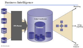
Data Warehouse is a central managed and integrated database containing data from the operational sources in an organization (such as SAP, CRM, ERP system). It may gather manual inputs from users determining criteria and parameters for grouping or classifying records.
That database contains structured data for query analysis and can be accessed by users. The data warehouse can be created or updated at any time, with minimum disruption to operational systems. It is ensured by a strategy implemented in a ETL process.

A source for the data warehouse is a data extract from operational databases. The data is validated, cleansed, transformed and finally aggregated and it becomes ready to be loaded into the data warehouse.
Data warehouse is a dedicated database which contains detailed, stable, non-volatile and consistent data which can be analyzed in the time variant.
Sometimes, where only a portion of detailed data is required, it may be worth considering using a data mart. A data mart is generated from the data warehouse and contains data focused on a given subject and data that is frequently accessed or summarized.


Keeping the data warehouse filled with very detailed and not efficiently selected data may lead to growing the database to a huge size, which may be difficult to manage and unusable. A good example of successful data management are set-ups used by the leaders in the field of telecoms such as O2 broadband. To significantly reduce number of rows in the data warehouse, the data is aggregated which leads to the easier data maintenance and efficiency in browsing and data analysis.

Key Data Warehouse systems and the most widely used database engines for storing and serving data for the enterprise business intelligence and performance management:
Teradata
SAP BW - Business Information Warehouse
Oracle
Microsoft SQL Server
IBM DB2
SAS
=====================================================================================
DataWarehouse Architecture

The main difference between the database architecture in a standard, on-line transaction processing oriented system (usually ERP or CRM system) and a DataWarehouse is that the system’s relational model is usually de-normalized into dimension and fact tables which are typical to a data warehouse database design.
The differences in the database architectures are caused by different purposes of their existence.

In a typical OLTP system the database performance is crucial, as end-user interface responsiveness is one of the most important factors determining usefulness of the application. That kind of a database needs to handle inserting thousands of new records every hour. To achieve this usually the database is optimized for speed of Inserts, Updates and Deletes and for holding as few records as possible. So from a technical point of view most of the SQL queries issued will be INSERT, UPDATE and DELETE.

Opposite to OLTP systems, a DataWarehouse is a system that should give response to almost any question regarding company performance measure. Usually the information delivered from a data warehouse is used by people who are in charge of making decisions. So the information should be accessible quickly and easily but it doesn't need to be the most recent possible and in the lowest detail level.

Usually the data warehouses are refreshed on a daily basis (very often the ETL processes run overnight) or once a month (data is available for the end users around 5th working day of a new month). Very often the two approaches are combined.

The main challenge of a DataWarehouse architecture is to enable business to access historical, summarized data with a read-only access of the end-users. Again, from a technical standpoint the most SQL queries would start with a SELECT statement.

In Data Warehouse environments, the relational model can be transformed into the following architectures:
Star schema
Snowflake schema
Constellation schema

Star schema architecture
Star schema architecture is the simplest data warehouse design. The main feature of a star schema is a table at the center, called the fact table and the dimension tables which allow browsing of specific categories, summarizing, drill-downs and specifying criteria.
Typically, most of the fact tables in a star schema are in database third normal form, while dimensional tables are de-normalized (second normal form).
Despite the fact that the star schema is the simpliest datawarehouse architecture, it is most commonly used in the datawarehouse implementations across the world today (about 90-95% cases).

Fact table
The fact table is not a typical relational database table as it is de-normalized on purpose - to enhance query response times. The fact table typically contains records that are ready to explore, usually with ad hoc queries. Records in the fact table are often referred to as events, due to the time-variant nature of a data warehouse environment.
The primary key for the fact table is a composite of all the columns except numeric values / scores (like QUANTITY, TURNOVER, exact invoice date and time).

Typical fact tables in a global enterprise data warehouse are (usually there may be additional company or business specific fact tables):

sales fact table - contains all details regarding sales
orders fact table - in some cases the table can be split into open orders and historical orders. Sometimes the values for historical orders are stored in a sales fact table.
budget fact table - usually grouped by month and loaded once at the end of a year.
forecast fact table - usually grouped by month and loaded daily, weekly or monthly.
inventory fact table - report stocks, usually refreshed daily

Dimension table
Nearly all of the information in a typical fact table is also present in one or more dimension tables. The main purpose of maintaining Dimension Tables is to allow browsing the categories quickly and easily.
The primary keys of each of the dimension tables are linked together to form the composite primary key of the fact table. In a star schema design, there is only one de-normalized table for a given dimension.

Typical dimension tables in a data warehouse are:

time dimension table
customers dimension table
products dimension table
key account managers (KAM) dimension table
sales office dimension table
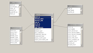
Star schema example
An example of a star schema architecture is depicted below.


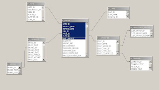
Snowflake Schema architecture
Snowflake schema architecture is a more complex variation of a star schema design. The main difference is that dimensional tables in a snowflake schema are normalized, so they have a typical relational database design.

Snowflake schemas are generally used when a dimensional table becomes very big and when a star schema can’t represent the complexity of a data structure. For example if a PRODUCT dimension table contains millions of rows, the use of snowflake schemas should significantly improve performance by moving out some data to other table (with BRANDS for instance).

The problem is that the more normalized the dimension table is, the more complicated SQL joins must be issued to query them. This is because in order for a query to be answered, many tables need to be joined and aggregates generated.

An example of a snowflake schema architecture is depicted below.


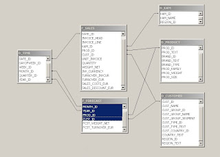
Fact constellation schema architecture
For each star schema or snowflake schema it is possible to construct a fact constellation schema.
This schema is more complex than star or snowflake architecture, which is because it contains multiple fact tables. This allows dimension tables to be shared amongst many fact tables.
That solution is very flexible, however it may be hard to manage and support.

The main disadvantage of the fact constellation schema is a more complicated design because many variants of aggregation must be considered.

In a fact constellation schema, different fact tables are explicitly assigned to the dimensions, which are for given facts relevant. This may be useful in cases when some facts are associated with a given dimension level and other facts with a deeper dimension level.
Use of that model should be reasonable when for example, there is a sales fact table (with details down to the exact date and invoice header id) and a fact table with sales forecast which is calculated based on month, client id and product id.
In that case using two different fact tables on a different level of grouping is realized through a fact constellation model.

An example of a constellation schema architecture is depicted below.

Fact constellation schema DW architecture

====================================================================================
Data mart
Data marts are designated to fulfill the role of strategic decision support for managers responsible for a specific business area.

Data warehouse operates on an enterprise level and contains all data used for reporting and analysis, while data mart is used by a specific business department and are focused on a specific subject (business area).

A scheduled ETL process populates data marts within the subject specific data warehouse information.

The typical approach for maintaining a data warehouse environment with data marts is to have one Enterprise Data Warehouse which comprises divisional and regional data warehouse instances together with a set of dependent data marts which derive the information directly from the data warehouse.

It is crucial to keep data marts consistent with the enterprise-wide data warehouse system as this will ensure that they are properly defined, constituted and managed. Otherwise the DW environment mission of being "the single version of the truth" becomes a myth. However, in data warehouse systems there are cases where developing an independent data mart is the only way to get the required figures out of the DW environment. Developing independent data marts, which are not 100% reconciled with the data warehouse environment and in most cases includes a supplementary source of data, must be clearly understood and all the associated risks must be identified.

Data marts are usually maintained and made available in the same environment as the data warehouse (systems like Oracle, Teradata, MS SQL Server, SAS) and are smaller in size than the enterprise data warehouse.
There are also many cases when data marts are created and refreshed on a server and distributed to the end users using shared drives or email and stored locally. This approach generates high maintenance costs, however makes it possible to keep data marts available offline.

There are two approaches to organize data in data marts:
Database datamart tables or its extracts represented by text files - one-dimensional, not aggregated data set; in most cases the data is processed and summarized many times by the reporting application.
Multidimensional database (MDDB) - aggregated data organized in multidimensional structure. The data is aggregated only once and is ready for business analysis right away.

In the next stage, the data from data marts is usually gathered by a reporting or analytic processing (OLAP) tool, such as Hyperion, Cognos, Business Objects, Pentaho BI, Microsoft Excel and made available for business analysis.

Usually, a company maintains multiple data marts serving the needs of finance, marketing, sales, operations, IT and other departments upon needs.

Example use of data marts in an organization: CRM reporting, customer migration analysis, production planning, monitoring of marketing campaigns, performance indicators, internal ratings and scoring, risk management, integration with other systems (systems which use the processed DW data) and more uses specific to the individual business.
================================================================================
SCD - Slowly changing dimensions
Slowly changing dimensions (SCD) determine how the historical changes in the dimension tables are handled. Implementing the SCD mechanism enables users to know to which category an item belonged to in any given date.

Types of Slowly Changing Dimensions in the Data Warehouse architectures:


Type 0 SCD is not used frequently, as it is classified as when no effort has been made to deal with the changing dimensions issues. So, some dimension data may be overwritten and other may stay unchanged over the time and it can result in confusing end-users.


Type 1 SCD DW architecture applies when no history is kept in the database. The new, changed data simply overwrites old entries. This approach is used quite often with data which change over the time and it is caused by correcting data quality errors (misspells, data consolidations, trimming spaces, language specific characters).
Type 1 SCD is easy to maintain and used mainly when losing the ability to track the old history is not an issue.


In the Type 2 SCD model the whole history is stored in the database. An additional dimension record is created and the segmenting between the old record values and the new (current) value is easy to extract and the history is clear. The fields 'effective date' and 'current indicator' are very often used in that dimension.


Type 3 SCD - only the information about a previous value of a dimension is written into the database. An 'old 'or 'previous' column is created which stores the immediate previous attribute. In Type 3 SCD users are able to describe history immediately and can report both forward and backward from the change.
However, that model can't track all historical changes, such as when a dimension changes twice or more. It would require creating next columns to store historical data and could make the whole data warehouse schema very complex.


Type 4 SCD idea is to store all historical changes in a separate historical data table for each of the dimensions.

In order to manage Slowly Changing Dimensions properly and easily it is highly recommended to use Surrogate Keys in the Data Warehouse tables.
A Surrogate Key is a technical key added to a fact table or a dimension table which is used instead of a business key (like product ID or customer ID).
Surrogate keys are always numeric and unique on a table level which makes it easy to distinguish and track values changed over time.

In practice, in big production Data Warehouse environments, mostly the Slowly Changing Dimensions Type 1, Type 2 and Type 3 are considered and used. It is a common practice to apply different SCD models to different dimension tables (or even columns in the same table) depending on the business reporting needs of a given type of data.

Reporting
A successful reporting platform implementation in a business intelligence environment requires great attention to be paid from both the business end users and IT professionals.
The fact is that the reporting layer is what business users might consider a data warehouse system and if they do not like it, they will not use it. Even though it might be a perfectly maintained data warehouse with high-quality data, stable and optimized ETL processes and faultless operation. It will be just useless for them, thus useless for the whole organization.

The problem is that the report generation process is not particularly interesting from the IT point of view as it does not involve heavy data processing and manipulation tasks. The IT professionals do not tend to pay great attention to this BI area as they consider it rather 'look and feel' than the 'real heavy stuff'.
From the other hand, the lack of technical exposure of the business users usually makes the report design process too complicated for them.
The conclusion is that the key to success in reporting (and the whole BI environment) is the collaboration between the business and IT professionals.

Types of reports
Reporting is a broad BI category and there is plenty of options and modes of its generation, definition, design, formatting and propagation.


The report types can be divided into several groups, illustrated below:
Standard, static report
Subject oriented, reported data defined precisely before creation
Reports with fixed layout defined by a report designer when the report is created
Very often the static reports contain subreports and perform calculations or implement advanced functions
Generated either on request by an end user or refreshed periodically from a scheduler
Usually are made available on the web server or a shared drive
Sample applications: Cognos Report Studio, Crystal Reports, BIRT
Ad-hoc report
Simple reports created by the end users on demand
Designed from scratch or using a standard report as a template
Sample applications: Cognos Analysis Studio
Interactive, multidimensional OLAP report
Usually provide more general information - using dynamic drill-down, slicing, dicing and filtering users can get the information they need
Reports with fixed design defined by a report designer
Generated either on request by an end user or refreshed periodically from a scheduler
Usually are made available on the web server or a shared drive
Sample applications: Cognos PowerPlay, Business Objects, Pentaho Mondrian
Dashboard
Contain high-level, aggregated company strategic data with comparisons and performance indicators
Include both static and interactive reports
Lots of graphics, charts, gauges and illustrations
Sample applications: Pentaho Dashboards, Oracle Hyperion, Microsoft SharePoint Server, Cognos Connection Portal
Write-back report
Those are interactive reports directly linked to the Data Warehouse which allow modification of the data warehouse data.
By far the most often use of this kind of reports is:
Editing and customizing products and customers grouping
Entering budget figures, forecasts, rebates
Setting sales targets
Refining business relevant data
Sample applications: Cognos Planning, SAP, Microsoft Access and Excel
Technical report
This group of reports is usually generated to fulfill the needs of the following areas:
IT technical reports for monitoring the BI system, generate execution performance statistics, data volumes, system workload, user activity etc.
Data quality reports - which are an input for business analysts to the data cleansing process
Metadata reports - for system analysts and data modelers
Extracts for other systems - formatted in a specific way
Usually generated in CSV or Microsoft Excel format
Reporting platforms
The most widely used reporting platforms:

IBM Cognos
SAP Business Objects and Crystal Reports
Oracle Hyperion and Siebel Analytics
Microstrategy
Microsoft Business Intelligence (SQL Server Reporting Services)
SAS
Pentaho Reporting and Analysis
BIRT - Open Source Business Intelligence and Reporting Tools
JasperReports
==================================================================================
Data mining
Data mining is an area of using intelligent information management tool to discover the knowledge and extract information to help support the decision making process in an organization. Data mining is an approach to discovering data behavior in large data sets by exploring the data, fitting different models and investigating different relationships in vast repositories.

The information extracted with a data mining tool can be used in such areas as decision support, prediction, sales forecasts, financial and risk analysis, estimation and optimization.

Sample real-world business use of data mining applications includes:

CRM - aids customers classification and retention campaigns
Web site traffic analysis - guest behavior prediction or relevant content delivery
Public sector organizations may use data mining to detect occurences of fraud such as money laundering and tax evasion, match crime and terrorist patterns, etc.
Genomics research - analysis of the vast data stores

The most widely known and encountered Data Mining techniques:
Statistical modeling which uses mathematical equations to do the analysis. The most popular statistical models are: generalized linear models, discriminant analysis, linear regression and logistic regression.
Decision list models and decision trees
Neural networks
Genetic algorithms
Screening models

Data mining tools offer a number data discovery techniques to provide expertise to the data and to help identify relevant set of attributes in the data:
Data manipulation which consists of construction of new data subsets derived from existing data sources.
Browsing, auditing and visualization of the data which helps identify non-typical, suspected relationships between variables in the data.
Hypothesis testing

A group of the most significant data mining tools is represented by:
SPSS Clementine
SAS Enterprise Miner
IBM DB2 Intelligent Miner
STATISTICA Data Miner
Pentaho Data Mining (WEKA)
Isoft Alice
==================================================================================
DATA FEDERATION
Try to remember all the times, when you had to collect data from many different sources. I guess, this reminds you all those situations when you have been searching and processing data for many hours, because you had to check every source one by one. After that it turns out that you had missed something and you spent another day attaching that missing data. However, there is solution, which can simplify your work. That solution is called “data federation”.

What is this and how does it work ?
Data federation is a kind of software that standardizes the integration of data from different (sometimes very dispersed) sources. It collects data from multiple sources, creates strategic layer of data and optimizes the integration of dispersed views, providing standardized access to those integrated view of information within single layer of data. That created layer ensures re-usability of the data. Due to that data federation has a very important significance while creating a SOA kind of software (Service Oriented Architecture - a computer system, where the main aim is to create software that will live up user’s expectations).


The most important advantages of good data federation software

Data federation strong points:
Large companies process huge amounts of data, that comes from different sources. In addition, with the company development, there are more and more data sources, that employees have to deal with and eventually it’s nearly impossible to work without using specific supportive software.
Standardized and simplified access to data – thanks to that even when we use data from different, dispersed sources that additionally have different formats, they can look like they are from the same source.
You can easily create integrated views of data and libraries of data store, that can be used multiple times.
Data are provided in real time, from original sources, not from cumulative databases or duplicates.
Efficient delivery of up-to-date data and protection of database in the same time.
Data federation weeknesses
There is no garden without weeds, so data federation also have some drawbacks.

While using that software, parameters should be closely watched and optimized, because aggregation logic takes place in server, not in the database. Wrong parameters or other errors can influence on the transmission or correctness of results. We should also remember that data comes from big amount of sources and it is important to check their reliability. Through using unproven and uncorrected data, we can have some errors in our work and that can cause financial looses for our company. Software can’t always judge if the source is reliable or not, so we have to make sure, that there ale special information managers, who watch over the correctness of data and decide what sources can our data federation application use.

As you can see, data federation system is very important, especially for big companies. It makes work with big amount of data from different sources much more easier.

Data federation - further reading on data federation
=====================================================================================
Data Warehouse metadata
The metadata in a data warehouse system unfolds the definitions, meaning, origin and rules of the data used in a Data Warehouse. There are two main types of metadata in a data warehouse system: business metadata and technical metadata. Those two types illustrate both business and technical point of view on the data.
The Data Warehouse Metadata is usually stored in a Metadata Repository which is accessible by a wide range of users.

Business metadata
Business metadata (datawarehouse metadata, front room metadata, operational metadata) - this type of metadata stores business definitions of the data, it contains high-level definitions of all fields present in the data warehouse, information about cubes, aggregates, datamarts.
Business metadata is mainly addressed to and used by the data warehouse users, report authors (for ad-hoc querying), cubes creators, data managers, testers, analysts.

Typically, the following information needs to be provided to describe business metadata:

DW Table Name
DW Column Name
Business Name - short and desctiptive header information
Definition - extended description with brief overiview of the business rules for the field
Field Type - a flag may indicate whether a given field stores the key or a discrete value, whether is active or not, or what data type is it. The content of that field (or fields) may vary upon business needs.


Technical metadata
Technical metadata (ETL process metadata, back room metadata, transformation metadata) is a representation of the ETL process. It stores data mapping and transformations from source systems to the data warehouse and is mostly used by datawarehouse developers, specialists and ETL modellers.
Most commercial ETL applications provide a metadata repository with an integrated metadata management system to manage the ETL process definition.
The definition of technical metadata is usually more complex than the business metadata and it sometimes involves multiple dependencies.

The technical metadata can be structured in the following way:

Source Database - or system definition. It can be a source system database, another data warehouse, file system, etc.
Target Database - Data Warehouse instance
Source Tables - one or more tables which are input to calculate a value of the field
Source Columns - one or more columns which are input to calculate a value of the field
Target Table - target DW table and column are always single in a metadata repository.
Target Column - target DW column
Transformation - the descriptive part of a metadata entry. It usually contains a lot of information, so it is important to use a common standard throughout the organisation to keep the data consistent.

Some tools dedicated to the metadata management(many of them are bundled with ETL tools):
Teradata Metadata Services
Erwin Data modeller
Microsoft Repository
IBM (Ascential) MetaStage
Pentaho Metadata
AbInitio EME (Enterpise Metadata Environment)
===================================================================================
Business Intelligence staffing
This study illustrates how global companies typically structure business intelligence resources and what teams and departments are involved in the support and maintenance of an Enterprise Data Warehouse.
This proposal may range widely across the organizations depending on the company requirements, the sector and BI strategy, however it might be considered as a template.

The successful business intelligence strategy requires the involvement of people from various departments. Those are mainly:
- Top Management (CIO, board of directors members, business managers)
- Finance
- Sales and Marketing
- IT - both business analysts and technical managers and specialists

Steering committee , Business owners
A typical enterprise data warehouse environment is under the control and direction of a steering committee. The steering committee sets the policy and strategic direction of the data warehouse and is responsible for the prioritization of the DW initiatives.
The steering committee is usually chaired by a DW business owner. Business owner acts as sponsor and champion of the whole BI environment in an organization.

Business Data Management group , Data governance team
This group forms the Business Stream of the BI staff and consist of a cross-functional team of representatives from the business and IT (mostly IT managers and analysts) with a shared vision to promote data standards, data quality, manage DW metadata and assure that the Data Warehouse is The Single Version of the Truth. Within the data governance group each major data branch has a business owner appointed to act as data steward. One of the key roles of the data steward is to approve access to the DW data.
The new DW projects and enhancements are shaped and approved by the Business Data Management group. The team also defines the Business Continuity Management and disaster recovery strategy.


Data Warehousing team
The IT stream of a Data Warehouse is usually the vastest and the most relevant from the technical perspective. It is hard to name this kind of team precisely and easily as it may differ significantly among organizations. This group might be referenced as Business Intelligence team, Data Warehousing team, Information Analysis Group, Information Delivery team, MIS Support, BI development, Datawarehousing Delivery team, BI solutions and services. Basically, the creativity of HR departments in naming BI teams and positions is much broader than you can imagine.
Some organizations also group the staff into smaller teams, oriented on a specific function or a topic.

The typical positions occupied by the members of the datawarehousing team are:

Data Warehouse analyst - those are people who know the OLTP and MIS systems and the dependencies between them in an organization. Very often the analysts create functional specification documents, high-level solution outlines, etc.
DW architect - a technical person which needs to understand the business strategy and implement that vision through technology
Business Intelligence specialist, Data Warehouse specialist, DW developer which are technical BI experts
ETL modeler, ETL developer - data integration technical experts
Reporting analyst, OLAP analyst , Information Delivery analyst, Report designer - people with analytical minds with some technical exposure
Team Leaders - by far the most often each of the Data Warehousing team subgroups has its own team leader who reports to a Business Intelligence IT manager. Those are very often experts who had been promoted.
Business Intelligence IT manager is a very important role because of the fact that a BI manager is a link between the steering committee, the data governance group and the experts.

DW Support and administration
This team is focused on the support, maintenance and resolution of operational problems within the data warehouse environment. The people included may be:

Database administrators (DBA)
Administrators of other BI tools in an organization (database, reporting, ETL)
Helpdesk support - customer support support the reporting front ends, accesses to the DW applications and other hardware and software problems

Sample DW team organogram
Enterprise Data Warehouse organizational chart with all the people involved and a sample staff count. The head count in our sample DW organization lists 35 people. Be aware that this organogram depends heavily on the company size and its mission, however it may be treated as a good illustration of proportions on the BI resources in a typical environment.
Keep in mind that not all positions involve full time resources.


Steering committee, Business owners - 3 *
Business Data Management group - 5
DW team - 20:
6 DW/ETL specialists and developers
3 report designers and analysts
6 DW technical analysts
5 Testers* (an analyst may also play the role of a tester)
Support and maintenance - 5*
===================================================================================
ETL process and concepts
ETL stands for extraction, transformation and loading. Etl is a process that involves the following tasks:

extracting data from source operational or archive systems which are the primary source of data for the data warehouse
transforming the data - which may involve cleaning, filtering, validating and applying business rules
loading the data into a data warehouse or any other database or application that houses data

The ETL process is also very often referred to as Data Integration process and ETL tool as a Data Integration platform.
The terms closely related to and managed by ETL processes are: data migration, data management, data cleansing, data synchronization and data consolidation.

The main goal of maintaining an ETL process in an organization is to migrate and transform data from the source OLTP systems to feed a data warehouse and form data marts.

ETL Tools
At present the most popular and widely used ETL tools and applications on the market are:


IBM Websphere DataStage (Formerly known as Ascential DataStage and Ardent DataStage)
Informatica PowerCenter
Oracle Warehouse Builder
Ab Initio
Pentaho Data Integration - Kettle Project (open source ETL)
SAS ETL studio
Cognos Decisionstream
Business Objects Data Integrator (BODI)
Microsoft SQL Server Integration Services (SSIS)

ETL process references
A detailed step-by-step instructions on how the ETL process can be implemented in IBM Websphere Datastage can be found in the Implementing ETL in DataStage tutorial lesson.

Etl process can be also successfully implemented using an open source ETL tool - Kettle. There is a separate Pentaho Data Integration section on our pages: Kettle ETL transformations