Data Build Tool (dbt )

 

dbt (data build tool) is a metadata-driven transformation framework that functions as a DAG-based SQL compiler and execution orchestrator for cloud data warehouses. Internally, it parses project files to construct a dependency graph using ref() and source(), then compiles Jinja-templated models into optimized SQL via its macro engine. Execution is delegated to the warehouse, with parallelization governed by graph topology. Core artifacts like manifest.json encode full lineage, configurations, and compiled nodes, while run_results.json captures execution telemetry. This architecture positions dbt as a control plane that unifies transformation logic, lineage, testing, and observability within modern data platforms.

What dbt Really Is (Architect Perspective)

At its core, dbt is a:

👉 Metadata-driven transformation framework
👉 SQL compiler + DAG execution engine
👉 Control plane over warehouse compute

Inside dbt Internals

• DAG
• Manifest.json
• Execution Engine

dbt is NOT a processing engine

• SQL Compiler + DAG Execution Framework

DAG Parsing

• dbt scans project files
• Builds dependency graph using ref()
• Creates Directed Acyclic Graph

Graph Structure

Each node =

• Model
• Test
• Seed

Each edge = dependency

👉 This drives execution order

manifest.json

The Brain of dbt

Contains:

• DAG structure
• Model metadata
• Compiled SQL
• Lineage

Why manifest.json Matters

• Powers dbt docs
• Enables lineage tools
• Integrates with DataHub / OpenLineage

Compilation Engine

Jinja SQL → Compiled SQL

Includes:

• Macros
• Variables
• Environment configs

Execution Model

dbt:
❌ Does NOT process data
✅ Pushes SQL to warehouse

Parallel execution based on DAG

run_results.json

Tracks:

• Execution status
• Runtime metrics
• Failures

👉 Used for observability

Architect Insight

If you understand:
✔ DAG
✔ manifest.json

👉 You understand dbt at scale

dbt = Metadata-driven transformation layer

Core vs Cloud vs Fusion — Strategic Comparison

 

How do you decide the number of executors, cores, and memory?

Rule-of-thumb (for a node with N cores, M GB RAM):

• Leave 1 core + ~1–2 GB for OS/overhead.
• Target 4–5 cores per executor (to limit GC overhead).
• Memory per executor: (node_memory - OS_reserve) / num_executors_per_node.
• Total executors = (#nodes * executors_per_node).
  Fine-tune by monitoring Spark UI: adjust if tasks are slow (need more cores/executors) or OOM (need more memory/fewer cores per executor).

 

What are the main components of a Spark cluster and how do they interact?

• Driver: Runs your main program, builds logical plans, coordinates tasks, holds metadata, sometimes collects results.
• Executors: JVM processes on worker nodes that run tasks, store cached data, and write shuffle files.
• Cluster manager (YARN / Kubernetes / Databricks / Standalone): Allocates resources (containers/pods/VMs) for driver and executors.
• Flow: Driver requests resources from cluster manager → cluster manager starts executors → driver sends tasks to executors and tracks progress.

IBM InfoSphere Change Data Capture

 
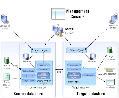
The key components of the InfoSphere CDC architecture are described below:

Access Server—Controls all of the non-command line access to the replication environment. When you log in to Management Console, you are connecting to Access Server. Access Server can be closed on the client workstation without affecting active data replication activities between source and target servers.
Admin API—Operates as an optional Java-based programming interface that you can use to script operational configurations or interactions.
Apply agent—Acts as the agent on the target that processes changes as sent by the source.  
Command line interface—Allows you to administer datastores and user accounts, as well as to perform administration scripting, independent of Management Console.  
Communication Layer (TCP/IP)—Acts as the dedicated network connection between the Source and the Target.  
Source and Target Datastore—Represents the data files and InfoSphere CDC instances required for data replication. Each datastore represents a database to which you want to connect and acts as a container for your tables. Tables made available for replication are contained in a datastore.  
Management Console—Allows you to configure, monitor and manage replication on various servers, specify replication parameters, and initiate refresh and mirroring operations from a client workstation. Management Console also allows you to monitor replication operations, latency, event messages, and other statistics supported by the source or target datastore. The monitor in Management Console is intended for time-critical working environments that require continuous analysis of data movement. After you have set up replication, Management Console can be closed on the client workstation without affecting active data replication activities between source and target servers.  
Metadata—Represents the information about the relevant tables, mappings, subscriptions, notifications, events, and other particulars of a data replication instance that you set up.  
Mirror—Performs the replication of changes to the target table or accumulation of source table changes used to replicate changes to the target table at a later time. If you have implemented bidirectional replication in your environment, mirroring can occur to and from both the source and target tables.
Refresh—Performs the initial synchronization of the tables from the source database to the target. This is read by the Refresh reader.  
Replication Engine—Serves to send and receive data. The process that sends replicated data is the Source Capture Engine and the process that receives replicated data is the Target Engine. An InfoSphere CDC instance can operate as a source capture engine and a target engine simultaneously.
Single Scrape—Acts as a source-only log reader and a log parser component. It checks and analyzes the source database logs for all of the subscriptions on the selected datastore.  
Source transformation engine—Processes row filtering, critical columns, column filtering, encoding conversions, and other data to propagate to the target datastore engine.  
Source database logs—Maintained by the source database for its own recovery purposes. The InfoSphere CDC log reader inspects these in the mirroring process, but filters out the tables that are not in scope for replication.  
Target transformation engine—Processes data and value translations, encoding conversions, user exits, conflict detections, and other data on the target datastore engine.

 There are two types of target-only destinations for replication that are not databases:  

JMS Messages—Acts as a JMS message destination (queue or topic) for row-level operations that are created as XML documents.  
InfoSphere DataStage—Processes changes delivered from InfoSphere CDC that can be used by InfoSphere DataStage jobs.

Applying change data by using a CDC Transaction stage

File organization input-output devices

File Oraganization can be sequential, line sequential, indexed, or relative.

Sequential file organization

The chronological order in which records are entered when a file is created establishes the arrangement of the records. Each record except the first has a unique predecessor record, and each record except the last has a unique successor record. Once established, these relationships do not change.
The access (record transmission) mode allowed for sequential files is sequential only.

Line-sequential file organization

Line-sequential files are sequential files that reside on the hierarchical file system (HFS) and that contain only characters as data. Each record ends with a new-line character. The only access (record transmission) mode allowed for line-sequential files is sequential.

Indexed file organization

Each record in the file contains a special field whose contents form the record key. The position of the key is the same in each record. The index component of the file establishes the logical arrangement of the file, an ordering by record key. The actual physical arrangement of the records in the file is not significant to your COBOL program. An indexed file can also use alternate indexes in addition to the record key. These keys let you access the file using a different logical ordering of the records. The access (record transmission) modes allowed for indexed files are sequential, random, or dynamic. When you read or write indexed files sequentially, the sequence is that of the key values.

Relative file organization

Records in the file are identified by their location relative to the beginning of the file. The first record in the file has a relative record number of 1, the tenth record has a relative record number of 10, and so on. The access (record transmission) modes allowed for relative files are sequential, random, or dynamic. When relative files are read or written sequentially, the sequence is that of the relative record number.

Sequential-only devices

Terminals, printers, card readers, and punches are called unit-record devices because they process one line at a time. Therefore, you must also process records one at a time sequentially in your program when it reads from or writes to unit-record devices. On tape, records are ordered sequentially, so your program must process them sequentially. Use QSAM physical sequential files when processing tape files. The records on tape can be fixed length or variable length. The rate of data transfer is faster than it is for cards.

Direct-access storage devices

Direct-access storage devices hold many records. The record arrangement of files stored on these devices determines the ways that your program can process the data. When using direct-access devices, you have greater flexibility within your program, because your can use several types of file organization:

# Sequential (VSAM or QSAM)
# Line sequential (UNIX)
# Indexed (VSAM)
# Relative (VSAM)

Choosing file organization and access mode

# If an application accesses records (whether fixed-length or variable-length) only sequentially and does not insert records between existing records, a QSAM or VSAM sequential file is the simplest type.
# If you are developing an application for UNIX that sequentially accesses records that contain only printable characters and certain control characters, line-sequential files work best.
# If an application requires both sequential and random access (whether records are fixed length or variable length), a VSAM indexed file is the most flexible type.
# If an application inserts and deletes records randomly, a relative file works well. Consider the following guidelines when choosing access mode:
# If a large percentage of a file is referenced or updated in an application, sequential access is faster than random or dynamic access.
# If a small percentage of records is processed during each run of an application, use random or dynamic access.

Note: courtesy of IBM

Netezza Enterprise Stage in DataStage

Netezza Enterprise stage is a database stage. You can use this stage to write bulk data to Netezza Performance Server(NPS). The Netezza Enterprise stage uses the Netezza write operator (nzwrite) to write data to Netezza Performance Server.

The Netezza write operator sets up a connection to an external data source and inserts records into a table. The operator takes a single input data set. The write mode determines how the records of a data set are inserted into the table.

Netezza write operator:

The Netezza write operator writes data to Netezza Performance Server. Netezza does not provide a read operator and hence the data retrieved from the source database is saved in a data set. The Netezza enterprise stage reads data from the data set and writes it to the Netezza Performance Server database.

Netezza data load methods:

The Netezza write operator employs two alternate methods to load data to Netezza Performance Server. You can write data to a Netezza Performance Server database either by using a nzload load utility or by writing data to an external table before writing it to the database.

nzload method:

You can use this load method if the data in the source database is consistent; that is, it implements a single character set for the entire database. Also the input schema for the nzload must be the same as that of the target table in the Netezza Performance Server database. The prerequisite to use the nzload method is that, nzclient utilities and ODBC functionality must be installed on the same computer as the IBM InfoSphere Information Server engine.

External table method:

If the data source that you want to read contains default values for table columns and uses variable format for data encoding such as UTF-8. You can write the data to an external table before loading it into the Netezza Performance Server database.

Write modes

Append:

Appends new rows to the specified table. To use this mode, you must have TABLE CREATE and INSERT privileges on the database that is being written to. Also the table must exist and the record schema of the data set must be compatible with the table. This mode is the default mode.

create

Creates a new table in the database. To use this mode, you must have TABLE CREATE privileges. If a table already exists with the same name as the one that you want to create, the step that contains this mode ends in error. The table is created with simple default properties. To create a table that is partitioned, indexed, in a non-default table space, or to create a customized table, you must use the -createstmt option with your own create table statement.

Replace

Drops the existing table and creates a new one in its place. To use this mode, you must have TABLE CREATE and TABLE DELETE privileges. If another table exists with the same name as the one that you want to create, the existing table is overwritten.

Truncate

Retains all the attributes of a table (including its schema), but discards the existing records and appends new records into the table. To use this mode, you must have DELETE and INSERT privileges on that table.

Netezza system

A Netezza system consists of multiple hardware and software components working together to provide performance and reliability. The NPS models include configurations with one or more hardware racks. Within each rack are numerous components that work together to provide the asymmetric massively parallel processing of the NPS architecture. The key hardware components within an NPS include the following:
􀁘 NPS Host
􀁘 Snippet Processing Units
􀁘 Snippet Processing Arrays

NPS Host

The NPS host, located within the NPS rack, controls and coordinates the activity of the NPS. It performs query optimization; controls table and database operations; consolidates and returns query results; and monitors the NPS system components to detect and report problems.

Snippet Processing Units

The Snippet Processing Unit (SPU) is the basic unit of processing and storage in the NPS.Each SPU is basically a standalone microcomputer, with a CPU, logic processors, memory,and disk storage.The SPU is an intelligent disk storage device, as it has logic to quickly search for the correct information and to return only the matching results of the portions of the data that are saved on its disk.An NPS system has many SPUs: up to 56,User database tables are distributed across all of the SPUs to allow for the parallel query processing.
Each SPU is responsible for managing a portion of your database and tables (called a primary partition), as well as for maintaining a copy of another SPU’s primary partition (called a mirror partition). If an SPU should fail, the mirror partition is used to create a new primary partition on a standby SPU within the system, which will then take the place of the failed SPU.

Snippet Processing Arrays

Snippet Processing Arrays (SPAs) are racks within the NPS system that contain up to 14 SPUs and have the power supplies, fans, and communication fabric that allows the SPUs to communicate with each other and with the NPS host. NPS systems contain at least two SPAs. If you add SPAs to the system to increase the number of SPUs, the SPAs are added in pairs. For each pair of SPAs, one of the 28 SPUs takes the role of a hot standby, ready to take the place of a failed SPU within the system.

NZSQL:

Commonly Used Command Options

nzload Command Options: